---
title: Non-Equilibrium Two Phase Flashing Flow Model Comparison
description: In contrast to the two-fluid models that require numerous assumptions and the corresponding closure equations, the simple model can be stated as... relief system design two phase flow process safety.
image: https://www.fauske.com/hubfs/Untitled-10.jpg
---

[![fauske-logo-white](https://www.fauske.com/hs-fs/hubfs/2024-website/branding/fauske-logo-white.png?width=181&height=32&name=fauske-logo-white.png) ](https://www.fauske.com/)

 Search on Fauske

[FAUSKE Line (+1-877-328-7531) ](tel:+18773287531)[ Test Cells & Accessories Store ](https://store.fauske.com/)[ Contact Us ](https://www.fauske.com/contact-us)

By Hans K. Fauske, D.Sc., Regent Advisor, Fauske & Associates, LLC

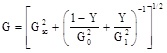
In contrast to the two-fluid models that require numerous assumptions and the corresponding closure equations, the simple model can be stated as:

![Untitled-11](https://www.fauske.com/hs-fs/hubfs/Untitled-11.jpg?width=167&name=Untitled-11.jpg) (1)

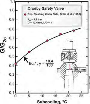
where G (kg m-2 s-1) is the two-phase flow rate including the effects of Subcooling (Gsc) and non-equilibrium, Y is the dimensionless independent variable ranging from 0 to 1 and G0 and G1 are the corresponding asymptotic flow rate limits. If all liquid exist at the stagnation condition, extensive data suggest that a simple length criterion L of the order of 100 mm characterizes the residence time requirement for approaching equilibrium flashing flow in ducts which are well described by the Equilibrium Rate Model (ERM), (Fauske, 1985). In this case Y in Eq. (1) represents the dimensionless length L+ = L/100 ranging from 0 to 1. For all specified stagnation conditions the easy to estimate G values with no arbitrary adjustable parameters are in remarkable agreement with available experimental data. An example is illustrated in Figure 1 comparing Eq. (1) with subcooled and saturated non-equilibrium flashing valve data.

**MODEL PREDICTIONS FOR FIGURE 1, FROM EQ. (1)**

**0 – Subcooling** saturated liquid at stagnation pressure P0 = 4.7 bar,![Untitled-1-19](https://www.fauske.com/hs-fs/hubfs/Untitled-1-19.jpg?width=47&name=Untitled-1-19.jpg)and the saturated flow limits are ![Untitled-2-5](https://www.fauske.com/hs-fs/hubfs/Untitled-2-5.jpg?width=321&name=Untitled-2-5.jpg) and ![Untitled-3-3](https://www.fauske.com/hs-fs/hubfs/Untitled-3-3.jpg?width=458&name=Untitled-3-3.jpg)  
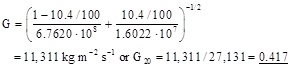
and the non-equilibrium flow rate from Eq. (1) is

![Untitled-4](https://www.fauske.com/hs-fs/hubfs/Untitled-4.jpg?width=293&name=Untitled-4.jpg)

is in excellent agreement with experimental data 0.42.

**5°C Subcooling** Tn = 144.5°C leads to a saturation pressure Ps = 4.0934 bar with P0 = 4.7 bar and  
![Untitled-6-1](https://www.fauske.com/hs-fs/hubfs/Untitled-6-1.jpg?width=356&name=Untitled-6-1.jpg) and the saturated liquid flow limits are  
![Untitled-7-1](https://www.fauske.com/hs-fs/hubfs/Untitled-7-1.jpg?width=362&name=Untitled-7-1.jpg)and  
![Untitled-8-1](https://www.fauske.com/hs-fs/hubfs/Untitled-8-1.jpg?width=473&name=Untitled-8-1.jpg)  
and the non-equilibrium two-phase flow rate from Eq. (1) is  
     ![Untitled-9-1](https://www.fauske.com/hs-fs/hubfs/Untitled-9-1.jpg?width=404&name=Untitled-9-1.jpg)  
            or G/G20 = 14,589/27,131 = 0.5397, in excellent agreement with experimental data = 0.54.

 ![Figure 1 - Crosby Safety Valve](https://www.fauske.com/hs-fs/hubfs/Untitled-10.jpg?width=300&name=Untitled-10.jpg)**References**

“Bolle, J. et al., 1995, “Flashing Water Flow Through a Safety Valve,” J. Loss   
     Prev. Process Ind. 8(2), p. 111 (1995).  
Fauske, H. K., 1985, “Flashing Flows: Some Practical Guidelines for Emergency  
     Releases,” Plant/Operation. Prog. 4(3), pp.132-134 (July 1985).

For more information regarding relief system design, two-phase flow and other [process safety engineering and testing](https://www.fauske.com/chemical-industry), please contact [info@fauske.com](mailto:info@fauske.com) or 630-323-8750

 

Figure 1

 

 

 

 [![Subscribe to Blog](https://no-cache.hubspot.com/cta/default/232514/657dbc54-1427-4b32-a2ad-f048135fc391.png)](https://cta-redirect.hubspot.com/cta/redirect/232514/657dbc54-1427-4b32-a2ad-f048135fc391)

```json
{
  "@context" : "https://schema.org",
  "@type" : "BlogPosting",
  "author" : {
    "@type" : "Person",
    "name" : "Fauske & Associates",
    "url" : "https://www.fauske.com/blog/author/fauske-and-associates"
  },
  "dateModified" : "2020-04-06T16:06:38.672Z",
  "datePublished" : "2018-08-28T00:52:00.000Z",
  "headline" : "Non-Equilibrium Two Phase Flashing Flow Model Comparison",
  "image" : [ "https://www.fauske.com/hubfs/Untitled-10.jpg" ],
  "mainEntityOfPage" : {
    "@id" : "https://www.fauske.com/blog/two-phase-flashing-flow-model-compared-to-safety-relief-valve-data",
    "@type" : "WebPage"
  },
  "publisher" : {
    "@type" : "Organization",
    "logo" : {
      "@type" : "ImageObject",
      "url" : "https://www.fauske.com/hubfs/FAUSKE-logo-Blue-Black-store-header-300px.png"
    },
    "name" : "Fauske & Associates"
  }
}
```

```json
// <![CDATA[
{
  "@context": "http://schema.org",
  "@type": "BlogPosting",
  "mainEntityOfPage": {
    "@type": "WebPage",
    "@id": "https://www.fauske.com/blog/two-phase-flashing-flow-model-compared-to-safety-relief-valve-data"
  },
  "headline": "A Simple and Accurate Non-Equilibrium Two Phase Flashing Flow Model Compared to Safety Relief Valve Data",
  "image": "https://cdn2.hubspot.net/hub/232514/hubfs/Untitled-10.jpg",
  "datePublished": "2018-08-27",
  "dateModified": "2018-08-28",
  "author": {
    "@type": "Person",
    "name": "Hans K. Fauske, D.Sc."
  },
   "publisher": {
    "@type": "Organization",
    "name": "Fauske & Associates, LLC",
    "logo": {
      "@type": "ImageObject",
      "url": "https://cdn2.hubspot.net/hub/232514/hubfs/Fauske-March%202017/Image/logo.jpg"
    }
  },
  "description": "In contrast to the two-fluid models that require numerous assumptions and the corresponding closure equations, the simple model can be stated as... relief system design two phase flow process safety."
}
// ]]>
```